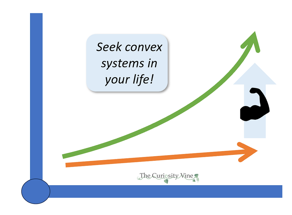
Just like someone does not need to be an auto mechanic to be a good car driver - you do not need to be a mathematician to create personal wealth! This article walks through the intuition behind a critical personal finance math concept called Jensen's Inequality and how investment transforms your savings.
About the author: Jeff Hulett is a behavioral economist and a decision scientist. He is an executive with the Definitive Companies. Jeff teaches personal finance and the decision sciences at James Madison University. Jeff is an author and his latest book is Making Choices, Making Money: Your Guide to Making Confident Financial Decisions. His experience includes senior leadership roles in banking and bank risk consulting. Jeff holds advanced degrees in finance, mathematics, and economics. Jeff and his family live in the Washington D.C. area.
Jensen's Inequality was first developed over one hundred years ago by Danish mathematician Johan Jensen. Its intuition is foundational to Personal Finance.
Here is the elegant mathematical version of Jensen's Inequality:
E[g(x)] >= g[E(x)]
iff g is CONVEX
------------------
g(x) is the transforming function
x is the set of inputs to g(x)
"Iff" means "If and only if."
"E[...]" means the "Expected value of..."
Another way to say Jensen's Inequality:
"For a convex function, the expected value of the function is always greater than or equal to the sum of the expected value of the individual parts of that function."
- or -
"The sum of the whole is worth more than the sum of its parts"
For a convex function:
This means the whole is greater than the sum of its parts.
This also means the value of what you get out of something is always greater than what you put into it.
Intuition to implement Jensen's Inequality
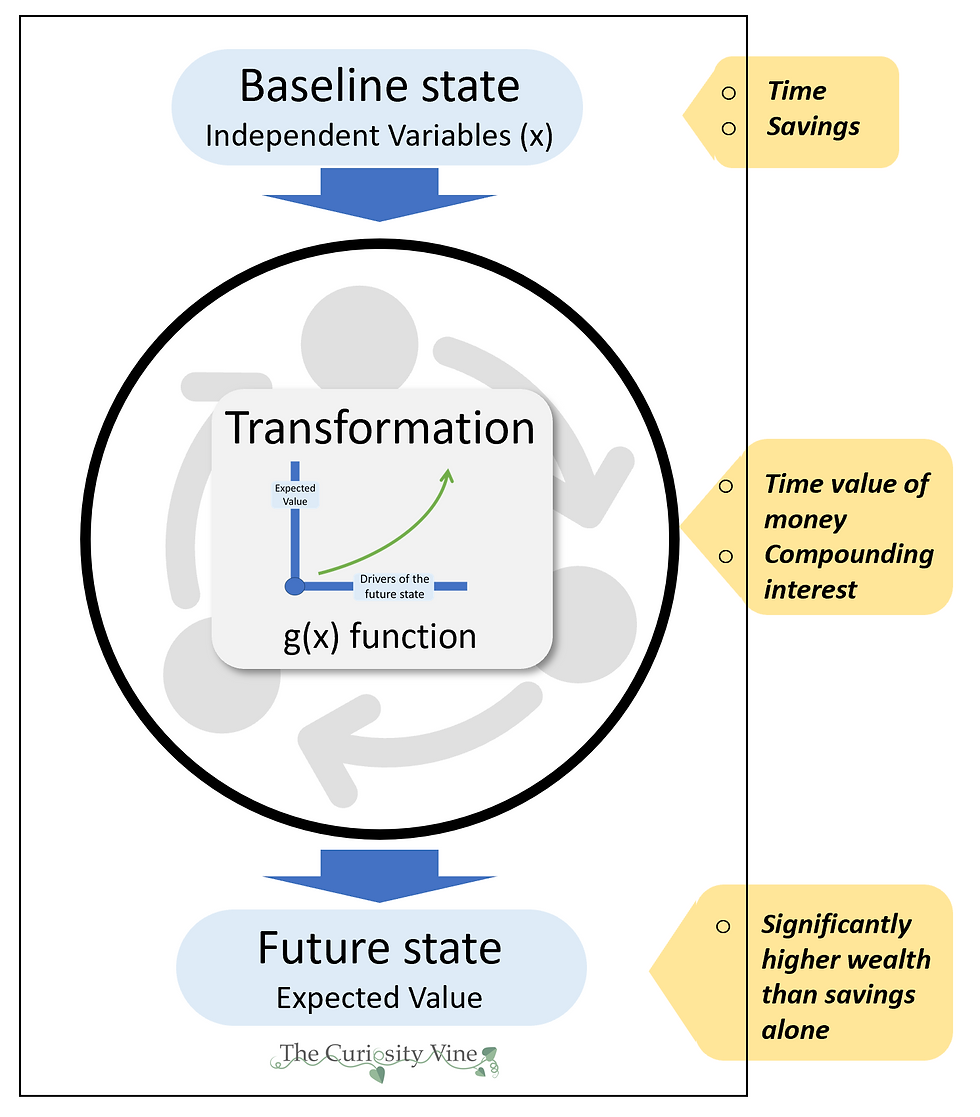
x or any other independent variables represents the baseline state. In the case of personal finance, the baseline is often time and your savings.
g(x) is the transforming function creating the new, future state. In the case of personal finance, the transformation will include a compounding interest rate.
The vertical axis (y) measures the Expected Value in the future state.
The horizontal axis (x) measures the drivers of that future state.
g(x), the transforming function, is convex to the drivers. For your savings, this means the expected value will grow at an increasing rate over time.
Convex functions are regenerative. It is good to seek convex systems to help transform your life. Exposing your savings to the convex compounding interest rate builds upon itself.
You can test convexity by drawing (or imagine drawing) all the tangent lines along the surface of g(x). If the set of all tangents falls on or BELOW g(x), then it is convex. Conversely, if the tangent lines are all on or ABOVE g(x), then the function is concave.

Simulation Example
For this example, a simple simulation model was developed to help explain Jensen's Inequality.
Imagine a fair die, with an equal probability of rolling a 1 to 6. Further, imagine a system providing a payoff that is the square of the die. Thus the system transforms the base state die into future payoffs different than the baseline. In this example, we use a squaring transformation function - x^2. The squaring function of the die system is CONVEX. Because the function is convex, Jensen's Inequality suggests the expected payout of the die system is always greater than or equal to that expected from the die alone. Next, shown is the math for this example:

Mean X = 3.5
(This is known as an Arithmetic Mean
"The sum of the parts"
Expected payoff from x = 12.25
(this is calculated as the mean of the x column, then squared.)
"The sum of the whole"
Expected payoff from x^2 = 15.16667
(this is calculated as the mean of x^2 column. This is known as a Geometric Mean)
Thus, per Jensen's Inequality:
15.2 > 12.25 and E[g(x)] >= g[E(x)]
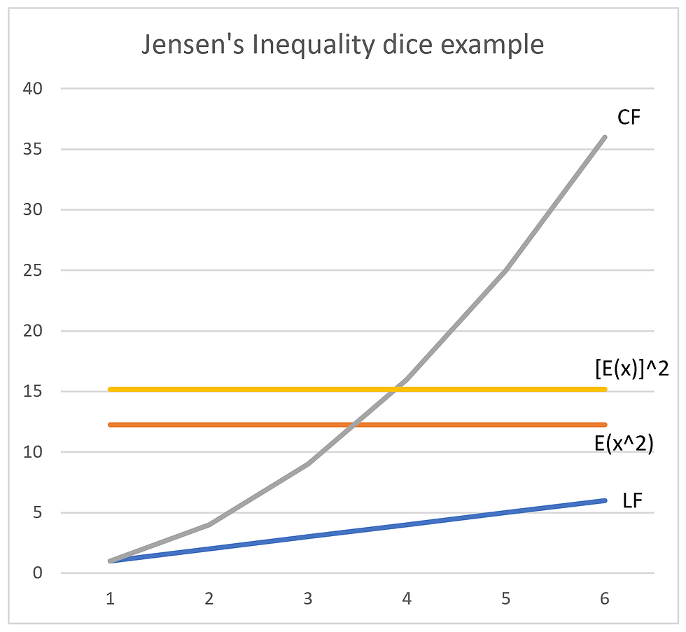
The expected value of the transformed convex function (CF) is always higher than the linear function (LF) from which it was transformed.
Please note: It is helpful to use simulations and visualizations to understand time-based transformation functions, such as those found in personal finance. There is efficiency and elegance in using personal finance math like Future Value or Annuity formulas. Certainly, mathematicians and financial engineers are taught to use formula-driven math in their work. However, the power of compounding and the subtle differences between arithmetic and geometric means are easy to lose without simulation and visualization. Fractal geometry, the mathematics of dynamical systems, is another example of where simulation and visualization are essential practitioner tools.
Jensen's Inequality is foundational for Personal Finance:
Next, we answer the "So What?!" question. How does this help us in our day-to-day life? The time value of money is an on-point example describing the power of Jensen's Inequality. Our regular savings is the baseline state. To get the most from the baseline state, it is necessary to make our savings a consistent, repeatable habit. Consistent savings alone, without any investment return, is a linear (not convex) function. Once savings are habituated, we wish to transform them into wealth. The transformation occurs via investments leveraging the time value of money. It is regenerative. It builds upon itself to help consistent savings grow. Compounding is the transforming function that moves linear savings to CONVEX wealth building. The essential driver is time. Your savings will grow over time if it is properly invested.
For more information on a proper investment approach, please see the article:
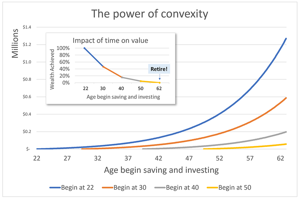
As an example, let's say you can consistently set aside $150 a month. This money is invested in a diversified securities portfolio that earns 10% a year over the long run. The idea is to save for your retirement. In this example, you wish to retire at age 62. The second-order questions are: "When should I start saving?" and "What is the impact of delaying savings?
The good news is that If you start at 22 and save 40 years until retirement, you will earn over $1.25mm for retirement.
But convexity is a double-edged sword.
Because the transformation function is convex to time, delay works against you in a big way. Just delaying 8 years, from 22 to 30, causes a significant decrease in potential retirement value. In this example, an 8-year delay causes you to lose almost $700k for retirement. As shown in the inset graphic, an 8-year delay from 22 to 30 years old causes you to lose over half your potential retirement savings. Note the blue line starts at 100% of the 22-year-old's $1.25mm in potential retirement value. As savings are delayed, the blue line drops to less than 50% of the potential retirement value at 30 years old.
The moral of the story is.... invest early and often! Even small amounts of savings will grow multiples over a longer time frame.
Please note: Elements of the time value of money are randomly determined. (aka "stochastic") For example, the 10% return discussed earlier is the expected average over time in the future. It is our best estimate based on past experience. It may be higher or lower in some years, depending on the economy and the investment markets. In general, for those saving for retirement, investing in well diversified, but higher volatility investment pools (like exchange-traded funds or ETFs) is suggested. This retirement investment strategy is discussed in the article:
It may be a bit uncomfortable that your investments are volatile. That is the price we pay for achieving a higher average return. In a longer timeframe like retirement, diversification protects your volatility from ruin. The nuances of risk and ruin are discussed in the article:
But what if you are already older than 22? Does this mean all is lost and you should not bother saving?
NO! Of course not! You will still benefit from the convex nature of the time value of money. Compare yourself to your older self. You will always do better by saving today instead of waiting until later.
Think like an economist! The past is sunk - the future is your playing field.
Connecting the dots - a personal finance transformation
Earlier we demonstrated the transformative power of convex functions and Jensen's Inequality. We showed this with a simple convex exponential function - x^2.
The time value of money is very similar. Next is the math notation for a common compounding interest function called FUTURE VALUE.

This is where:
FV - Future Value of your investment at the end of the time period.
PV - Present Value of your savings at the beginning of the time period.
r - interest rate
n - number of years or time periods
Notice, this formula is similar to our earlier x^2 function. The essential similarity is the exponential nature of time, n. The future value function is also convex! This future value formula underlies the earlier graphic. This is how $150 of monthly savings is transformed to make you a millionaire by the time you retire.
Showing graphically how convex functions operate over time is essential to conveying the power of convexity to transform savings - and your life. While the future value "end number" is more compact and possibly more mathematically elegant, it is the visual that shows how time and savings transform your life.
Please see this article for a personal finance example of Jensen's Equality in action!
But life and investing has its ups and downs. How does convexity impact life's volatility?
This is an important question. Convexity does not promise your investments will increase every day. The idea of convexity is that volatility will hurt you less to the downside and help you more to the upside in the long run and in a well-diversified portfolio. The annual investment return we use for the previous example is a long-term average. Keep in mind, on paper, you will see losses or gains owing to market volatility every day. Stock prices go up and down all the time! This is normal. Being convex to time is your superpower. This means, over time the downside risks will hurt you less than the upside benefits of that volatility. Notice, the words "well-diversified," this is how you protect yourself from ruin. If one of the companies fails, your diversification enables you to return. No one company creates ruin risk for a well-diversified portfolio.
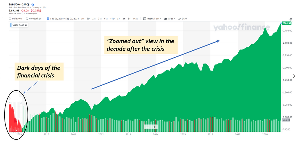
Next is an example of the benefits of being convex to time. The great financial crisis of 2007-2008 is an example of significant downside volatility risk. This graphic is an example of how downside volatility risk was overcome by the upside volatility benefit, EVEN AFTER THE GREATEST FINANCIAL CRISIS SINCE THE GREAT DEPRESSION. Another way to look at it -- do NOT think of volatility risk as being good or bad. Volatility risk WILL happen in any well-functioning market. The crux move is being CONVEX TO TIME to properly manage a well-diversified portfolio. The challenge, then, is how to stay in the game, even when the market is creating. This is the domain of commitment devices, like auto transfer, to make sure your investment strategy is operating in a market down drafts. As Nobel laureate and University of Chicago behavior economist Richard Thaler said:
"There is growing evidence that most people would be better off not paying attention to the ebbs and flows of the stock market.”
For more information, please see the article:
Please note: This is an example of how to:
Take a single non-ergodic "time is NOT your friend" company and
Use diversification to have it behave more like an ergodic "time IS your friend" portfolio.

Comments